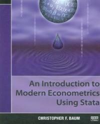
An Introduction to Modern Econometrics Using Stata, by Christopher F. Baum, successfully bridges the gap between learning econometrics and learning how to use Stata. The book presents a contemporary approach to econometrics, emphasizing the role of method-of-moments estimators, hypothesis testing, and specification analysis while providing practical examples showing how the theory is applied to real datasets by using Stata. The first three chapters are dedicated to the basic skills needed to effectively use Stata: loading data into Stata; using commands like generate and replace, egen, and sort to manipulate variables; taking advantage of loops to automate tasks; and creating new datasets by using merge and append. Baum succinctly yet thoroughly covers the elements of Stata that a user must learn to become proficient, providing many examples along the way. Chapter 4 begins the core econometric material of the book and covers the multiple linear regression model, including efficiency of the ordinary least-squares estimator, interpreting the output from regress, and point and interval prediction. The chapter covers both linear and nonlinear Wald tests, as well as constrained least-squares estimation, Lagrange multiplier tests, and hypothesis testing of nonnested models. Chapters 5 and 6 focus on consequences of failures of the linear regression model’s assumptions. Chapter 5 addresses topics like omitted-variable bias, misspecification of functional form, and outlier detection. Chapter 6 is dedicated to non-independently and identically distributed errors, and it introduces the Newey–West and Huber/White covariance matrices, as well as feasible generalized least-squares estimation in the presence of heteroskedasticity or serial correlation. Chapter 7 is dedicated to the use of indicator variables and interaction effects. Instrumental-variables estimation has been an active area of research in econometrics, and chapter 8 commendably addresses issues like weak instruments, underidentification, and generalized method-of-moments estimation. In this chapter, Baum extensively uses his wildly popular ivreg2 command. The last two chapters briefly introduce panel-data analysis and discrete and limited-dependent variables. Two appendices detail importing data into Stata and Stata programming. As in all chapters, Baum presents many Stata examples. An Introduction to Modern Econometrics Using Stata can serve as a supplementary text in both undergraduate- and graduate-level econometrics courses, and the book’s examples will help students quickly become proficient in Stata. The book is also useful to economists and businesspeople wanting to learn Stata by using practical examples.

Illustrations Preface Notation and typography 1 Introduction 1.1 An overview of Stata’s distinctive features 1.2 Installing the necessary software 1.3 Installing the support materials 2 Working with economic and financial data in Stata 2.1 The basics 2.1.1 The use command 2.1.2 Variable types 2.1.3 _n and _N 2.1.4 generate and replace 2.1.5 sort and gsort 2.1.6 if exp and in range 2.1.7 Using if exp with indicator variables 2.1.8 Using if exp versus by varlist: with statistical commands 2.1.9 Labels and notes 2.1.10 The varlist 2.1.11 drop and keep 2.1.12 rename and renvars 2.1.13 The save command 2.1.14 insheet and infile 2.2 Common data transformations 2.2.1 The cond() function 2.2.2 Recoding discrete and continuous variables 2.2.3 Handling missing data mvdecode and mvencode 2.2.4 String-to-numeric conversion and vice versa 2.2.5 Handling dates 2.2.6 Some useful functions for generate or replace 2.2.7 The egen command Official egen functions egen functions from the user community 2.2.8 Computation for by-groups 2.2.9 Local macros 2.2.10 Looping over variables: forvalues and foreach 2.2.11 Scalars and matrices 2.2.12 Command syntax and return values 3 Organizing and handling economic data 3.1 Cross-sectional data and identifier variables 3.2 Time-series data 3.2.1 Time-series operators 3.3 Pooled cross-sectional time-series data 3.4 Panel data 3.4.1 Operating on panel data 3.5 Tools for manipulating panel data 3.5.1 Unbalanced panels and data screening 3.5.2 Other transforms of panel data 3.5.3 Moving-window summary statistics and correlations 3.6 Combining cross-sectional and time-series datasets 3.7 Creating long-format datasets with append 3.7.1 Using merge to add aggregate characteristics 3.7.2 The dangers of many-to-many merges 3.8 The reshape command 3.8.1 The xpose command 3.9 Using Stata for reproducible research 3.9.1 Using do-files 3.9.2 Data validation: assert and duplicates 4 Linear regression 4.1 Introduction 4.2 Computing linear regression estimates 4.2.1 Regression as a method-of-moments estimator 4.2.2 The sampling distribution of regression estimates 4.2.3 Efficiency of the regression estimator 4.2.4 Numerical identification of the regression estimates 4.3 Interpreting regression estimates 4.3.1 Research project: A study of single-family housing prices 4.3.2 The ANOVA table: ANOVA F and R-squared 4.3.3 Adjusted R-squared 4.3.4 The coefficient estimates and beta coefficients 4.3.5 Regression without a constant term 4.3.6 Recovering estimation results 4.3.7 Detecting collinearity in regression 4.4 Presenting regression estimates 4.4.1 Presenting summary statistics and correlations 4.5 Hypothesis tests, linear restrictions, and constrained least squares 4.5.1 Wald tests with test 4.5.2 Wald tests involving linear combinations of parameters 4.5.3 Joint hypothesis tests 4.5.4 Testing nonlinear restrictions and forming nonlinear combinations 4.5.5 Testing competing (nonnested) models 4.6 Computing residuals and predicted values 4.6.1 Computing interval predictions 4.7 Computing marginal effects 4.A Appendix: Regression as a least-squares estimator 4.B Appendix: The large-sample VCE for linear regression 5 Specifying the functional form 5.1 Introduction 5.2 Specification error 5.2.1 Omitting relevant variables from the model Specifying dynamics in time-series regression models 5.2.2 Graphically analyzing regression data 5.2.3 Added-variable plots 5.2.4 Including irrelevant variables in the model 5.2.5 The asymmetry of specification error 5.2.6 Misspecification of the functional form 5.2.7 Ramsey's RESET 5.2.8 Specification plots 5.2.9 Specification and interaction terms 5.2.10 Outlier statistics and measures of leverage The DFITS statistic The DFBETA statistic 5.3 Endogeneity and measurement error 6 Regression with non-i.i.d. errors 6.1 The generalized linear regression model 6.1.1 Types of deviations from i.i.d. errors 6.1.2 The robust estimator of VCE 6.1.3 The cluster estimator of VCE 6.1.4 The Newey–West estimator of VCE 6.1.5 The generalized-least squares estimator The FGLS estimator 6.2 Heteroskedasticity in the error distribution 6.2.1 Heteroskedasticity related to scale Testing for heteroskedasticity related to scale FGLS estimation 6.2.2 Heteroskedasticity between groups of observations Testing for heteroskedasticity between groups of observations FGLS estimation 6.2.3 Heteroskedasticity in grouped data FGLS estimation 6.3 Serial correlation in the error distribution 6.3.1 Testing for serial correlation 6.3.2 FGLS estimation with serial correlation 7 Regression with indicator variables 7.1 Testing for significance of a qualitative factor 7.1.1 Regression with one qualitative measure 7.1.2 Regression with two qualitative measures Interaction effects 7.2 Regression with qualitative and quantitative factors Testing for slope differences 7.3 Seasonal adjustment with indicator variables 7.4 Testing for structural stability and structural change 7.4.1 Constraints of continuity and differentiability 7.4.2 Structural change in a time-series model 8 Instrumental-variables estimators 8.1 Introduction 8.2 Endogeneity in economic relationships 8.3 2SLS 8.4 The ivreg command 8.5 Identification and tests of overidentifying restrictions 8.6 Computing IV estimates 8.7 ivreg2 and GMM estimation 8.7.1 The GMM estimator 8.7.2 GMM in a homoskedastic context 8.7.3 GMM and heteroskedasticity-consistent standard errors 8.7.4 GMM and clustering 8.7.5 GMM and HAC standard errors 8.8 Testing and overidentifying restrictions in GMM 8.8.1 Testing a subset of the overidentifying restrictions in GMM 8.9 Testing for heteroskedasticity in the IV context 8.10 Testing the relevance of instruments 8.11 Durbin–Wu–Hausman tests for endogeneity in IV estimation 8.A Appendix: Omitted-variables bias 8.B Appendix: Measurement error 8.B.1 Solving errors-in-variables problems 9 Panel-data models 9.1 FE and RE models 9.1.1 One-way FE 9.1.2 Time effects and two-way FE 9.1.3 The between estimator 9.1.4 One-way RE 9.1.5 Testing the appropriateness of RE 9.1.6 Prediction from one-way FE and RE 9.2 IV models for panel data 9.3 Dynamic panel-data models 9.4 Seemingly unrelated regression models 9.4.1 SUR with identical regressors 9.5 Moving-window regression estimates 10 Models of discrete and limited dependent variables 10.1 Binomial logit and probit models 10.1.1 The latent-variable approach 10.1.2 Marginal effects and predictions Binomial probit Binomial logit and grouped logit 10.1.3 Evaluating specification and goodness of fit 10.2 Ordered logit and probit models 10.3 Truncated regression and tobit models 10.3.1 Truncation 10.3.2 Censoring 10.4 Incidental truncation and sample-selection models 10.5 Bivariate probit and probit with selection 10.5.1 Binomial probit with selection A Getting the data into Stata A.1 Inputting data from ASCII text files and spreadsheets A.1.1 Handling text files Free format versus fixed format The insheet command A.1.2 Accessing data stored in spreadsheets A.1.3 Fixed-format data files A.2 Importing data from other package formats B The basics of Stata programming B.1 Local and global macros B.1.1 Global macros B.1.2 Extended macro functions and list functions B.2 Scalars B.3 Loop constructs B.3.1 foreach B.4 Matrices B.5 return and ereturn B.5.1 ereturn list B.6 The program and syntax statements B.7 Using Mata functions in Stata programs References Author index Subject index